Dijkstra's Algorithm: The Backbone of GPS Navigation
Imagine you are standing in a city with thousands of intersecting roads, being asked to determine the fastest route to every possible destination without wasting a single step. Solving that problem efficiently requires more than intuition; it requires structure.
Graph Theory
Graph theory is the study of graphs and is a branch of mathematics. Specifically, it focuses on the analysis of connections in networks using nodes (points on the graph) and connections between them. In weighted graphs, edges—the paths that lead to neighboring nodes—are assigned numerical values (weights), often representing the cost or time of traveling between nodes. Using weighted graphs, algorithms can optimize weights to find ideal paths.
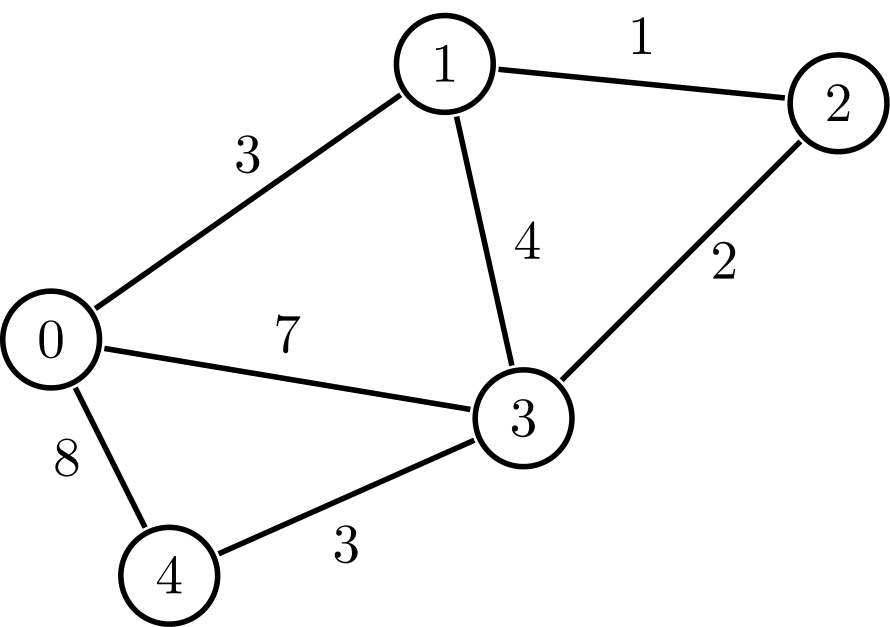
An example of a graph with 5 nodes (the circles) numbered 0-4, and 7 edges (the paths between them) with each edge’s respective weight.
The Conception of Dijkstra’s Algorithm
Dijkstra’s algorithm, conceived by computer scientist Edsger W. Dijkstra in 1956, is an algorithm in graph theory that finds the shortest paths from a single node in a weighted graph. Dijkstra’s algorithm ultimately finds the most weight-optimized path from a single starting node to all other nodes in the graph. In other words, it’s a one-way network of nodes in which only the shortest paths exist.
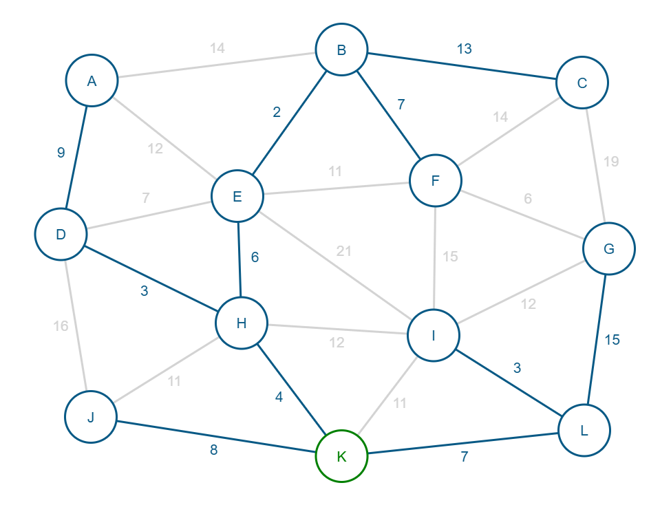
An example of a Dijkstra-optimized graph where node K (the green circle) was the starting node.
How Dijkstra’s Algorithm Works
Dijkstra’s algorithm utilizes a greedy principle, the process of systematically exploring a graph to find the shortest possible paths using a priority queue. Priority queuesmanage which nodes to visit next, always selecting the unvisited node with the smallest known distance from the source. You can also think of priority queues this way: it’s like a waiting room where the person with the most urgent need—in this case, the closest node from the start node—is served next, regardless of when they arrived.
The core process involves the following steps:
Initialization: Assign a distance of 0 to the starting node and an initial distance of infinity to all other nodes. All nodes are marked as unvisited.
We initialize all other nodes with a distance of infinity because any other path must be compared against a previously recorded path. At the start, no such comparison exists. By assigning infinity as the initial value, the first discovered path will always be accepted as the shortest known path up to that point.
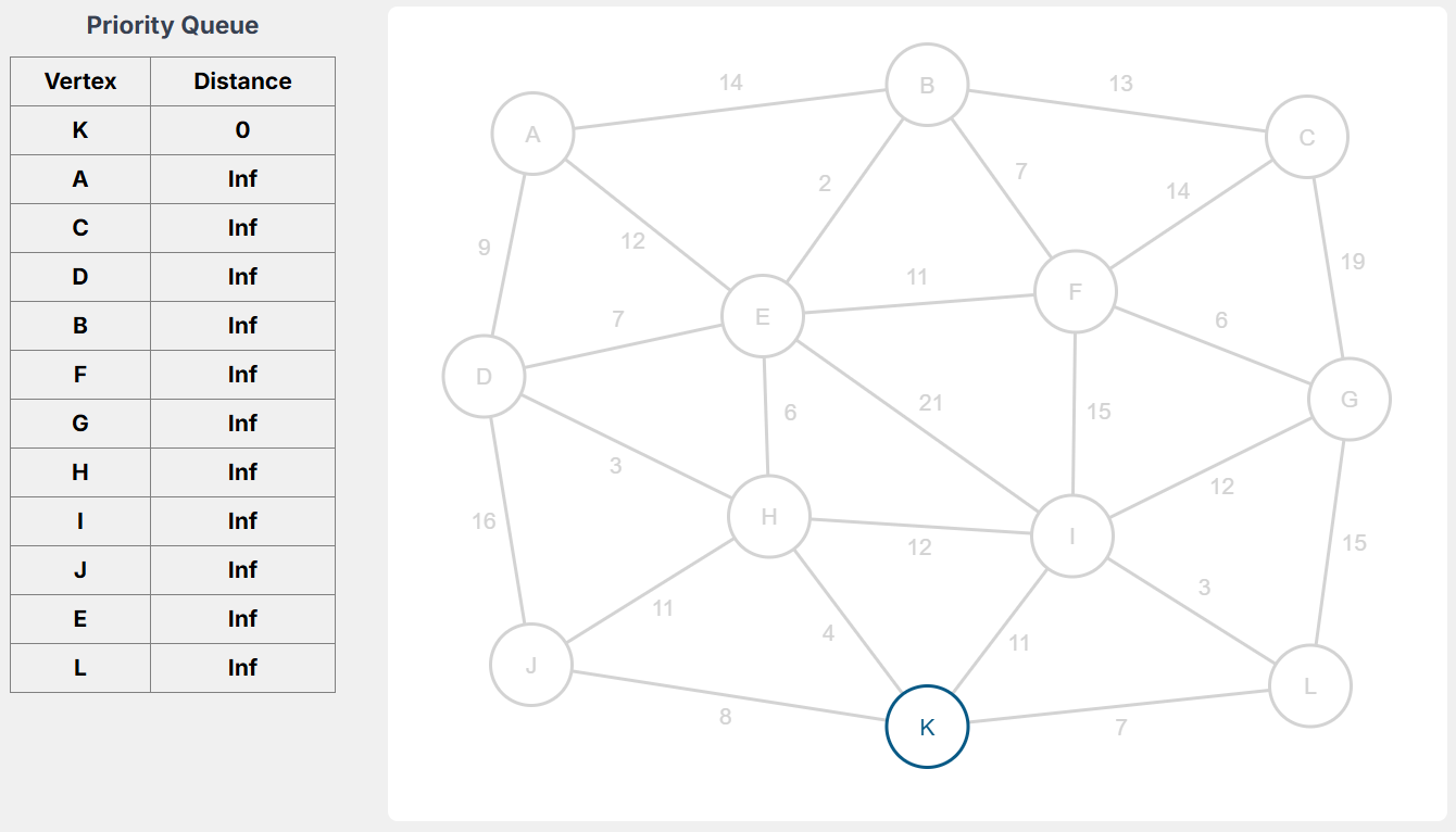
An example of an initialized priority queue, in which K (the blue circle) is the starting node, and thus it is also the first selected node for exploration. However, the algorithm has not begun searching yet.
Selection: Select the unvisited node with the smallest tentative distance from the source.
In other words, you’re asserting that the current recorded path to the selected node is the shortest path known so far. However, this does not guarantee the globally optimal path, since a shorter path may still be discovered later in the algorithm’s execution.
If you’re having trouble understanding what tentative distance is. Think of it like this: “this is the shortest path based on what I know so far, but it’s possible that a shorter path exists.“
Exploration (Relaxation): Mark the selected node as “visited”. For all its unvisited neighbors, calculate the length of their paths from the source through the current node. If this newly calculated path is shorter than their current path, update their distance.
During the exploration phase, each neighboring node’s distance is computed and compared to its current recorded distance to determine whether a shorter path has been found. Importantly, the neighbor is not immediately marked as “visited,” as it allows the algorithm to revisit and update it if a shorter path emerges later.
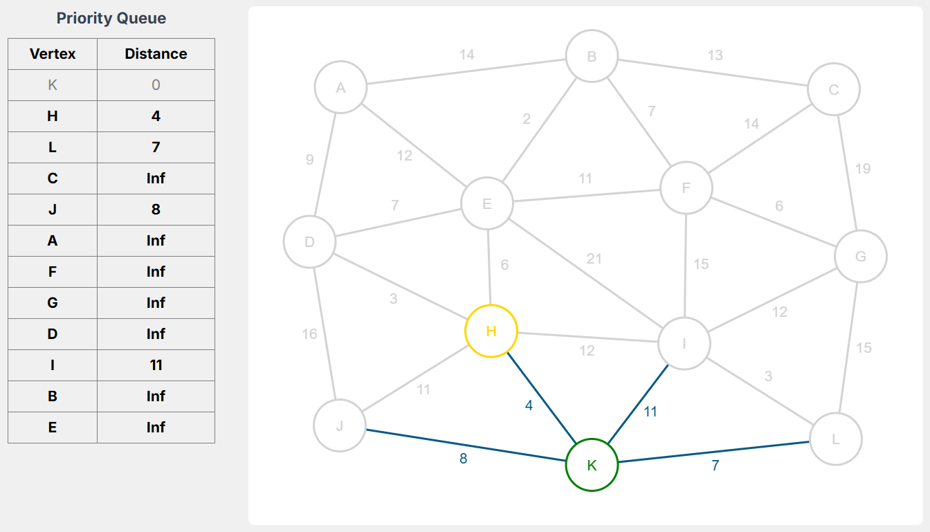
In this updated graph, node K has been fully searched and the algorithm is now moving on to the next node. Note that the paths of the neighbors of node K have been updated to reflect their current tentative distance.
Repetition: Repeat selection and exploration until all nodes have been visited or the destination node is reached. If you’re only finding a single destination path, Dijkstra’s technically does not need to fully execute, as it’s designed to run until it finds the shortest path to every node.
At this stage, nodes are marked as “visited.” A node is only marked as visited once its shortest possible distance has been finalized—meaning all incoming paths (paths that lead into the node) have been considered (passed through). At that point, the node is regarded as fully explored and will not be revisited.
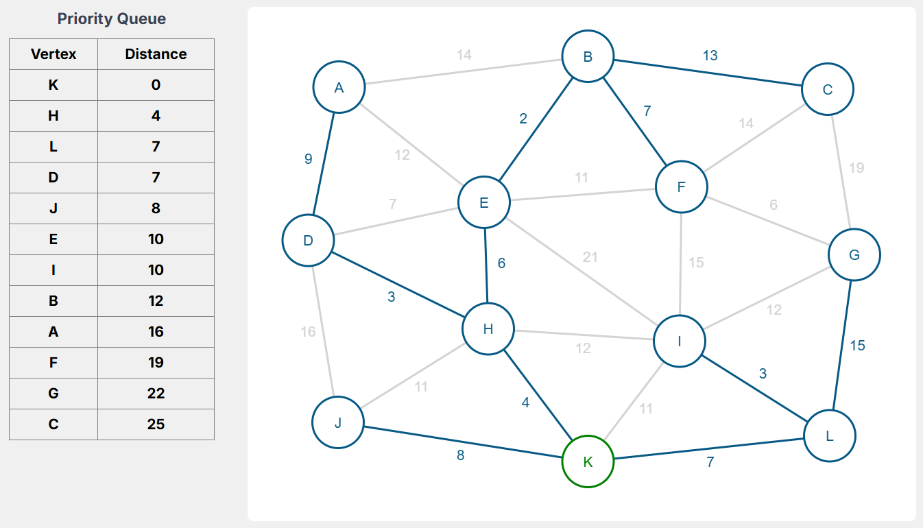
This is the fully optimized version of the graph after Dijkstra’s algorithm. Notice that the initial path to node I has changed, now passing through node L because it’s a shorter distance. This exemplifies tentative distance.
Dijkstra’s Algorithm And Negative Weights
Now that you know the functionality of Dijkstra’s algorithm, you should realize that it only guarantees an optimal solution if all edge weights in the graph are non-negative. For graphs with negative edge weights, a different algorithm, such as the Bellman-Ford algorithm, must be used.
If you’re wondering why, the answer is simple. Remember how Dijkstra’s algorithm relies on a greedy principle? Well this foundation assumes that adding an edge can never make a path shorter. However, this assumption only holds if you are traversing edges that can’t reduce the total path distance—which is only true when all edge weights are positive and add to the total distance.
That's why picking the shortest edge locally always ends up being correct globally in a non-negative weighted graph. A negative edge weight breaks a greedy principle’s fundamental assumption. A path that initially appears longer might use a negative edge later to become the true shortest path to a previously "visited" node.
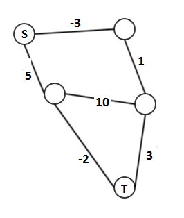
For example, in an initial run of this graph, a greedy principle assumes that the weight of 3 (-2+5)—consisting of 2 edges—is the shortest path from T to S.
However, later in the algorithm, we find that the true shortest path is 1 (3+1-3)—using 3 edges—which violates the greedy principle’s assumption.
Dijkstra’s Algorithm and Real-world Applications
Dijkstra’s algorithm is widely used across various industries due to its efficiency and reliability. Such industries include, but are not limited to:
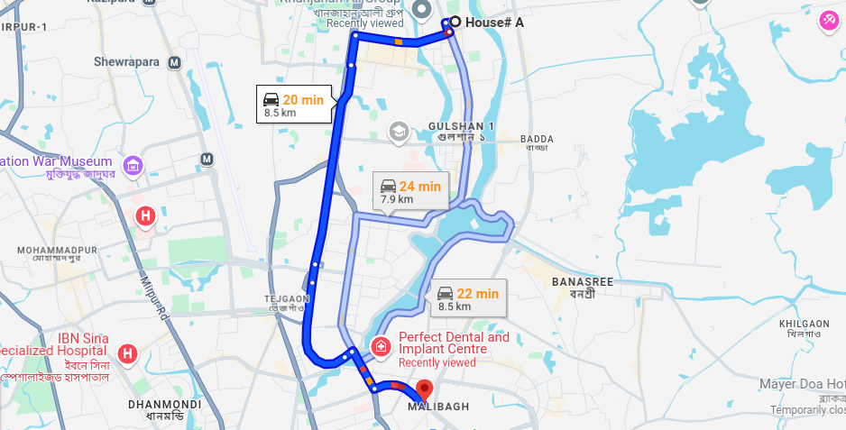
Navigation Systems: Applications like Google Maps use Dijkstra's algorithm to calculate the shortest driving route between locations, considering factors like distance and traffic.
Network Routing: It’s a key component in internet routing protocols like OSPF (Open Shortest Path First), helping routers determine the most efficient path for data packets to traverse and minimizing latency.
Logistics and Transportation: Companies use it to optimize delivery routes, reduce costs, and improve efficiency in supply chain management.
Social Networks: It can be used to find the shortest degree of separation (number of handshakes/connections) between users.